Just how accurate is your Einstein AI model?

Explaining Einstein Discovery Model Metrics

The clever people at Salesforce have made it relatively straightforward to build and deploy a predictive data model via their supervised machine-learning platform, Einstein.

Now, as you build and test your Einstein AI models, you need to be able assess how accurate and trustworthy your predictions are. Fortunately, Salesforce has built a mechanism for doing so into their platform – “Model Metrics”:

Here is an example; note that a logistic regression model would have two more tabs:

Now, I think that many of you, depending upon your training and background, might not recognise all of these metrics. I know that I didn’t when I first saw them!

I have provided an overview below of the meaning of these twelve terms. Please consult my references at the bottom of the post for more detailed information. Feedback is welcomed!

1. MSE – Mean Squared Error

Mean Squared Error is a measure of how close a fitted line is to data points. For every data point, you take the distance vertically from the point to the corresponding y value on the curve fit (the error) and square the value. Then you add up all those values for all data points, and, in the case of a fit with two parameters such as a linear fit, divide by the number of points minus two. The squaring is done so negative values do not cancel positive values. The smaller the Mean Squared Error, the closer the fit is to the data.

The “squared” bit means the bigger the error, the more it is punished. If your correct answers are 2,3,4 and your algorithm guesses 1,4,3, the absolute error on each one is exactly 1, so squared error is also 1, and the MSE is 1. But if your algorithm guesses 2,3,6, the errors are 0,0,2, the squared errors are 0,0,4, and the MSE is a higher 1.333.

2. RMSE – Root Mean Squared Error

The Root Mean Squared Error is just the square root of the mean square error. That is probably the most easily interpreted statistic, since it has the same units as the quantity plotted on the vertical axis. The RMSE is thus the distance, on average, of a data point from the fitted line, measured along a vertical line. The RMSE is directly interpretable in terms of measurement units, and so is a better measure of goodness of fit than a correlation coefficient. One can compare the RMSE to observed variation in measurements of a typical point. The two should be similar for a reasonable fit.

3. Number of Observations

Sample size determination is the act of choosing the number of observations or replicates to include in a statistical sample. The sample size is an important feature of any empirical study in which the goal is to make inferences about a population from a sample. In practice, the sample size used in a study is determined based on the expense of data collection, and the need to have sufficient statistical power.

The general rule of thumb is that if you expect to be able to detect reasonable-size effects with reasonable power, you need 10-20 observations per parameter (covariate) estimated.

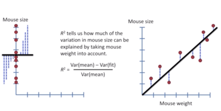
4. R Squared

R-squared is a statistical measure of how close the data are to the fitted regression line. It is also known as the coefficient of determination, or the coefficient of multiple determination for multiple regression. The definition of R-squared is fairly straight-forward; it is the percentage of the response variable variation that is explained by a linear model. Or:

R-squared = Explained variation / Total variation

R-squared is always between 0 and 100%:

0% indicates that the model explains none of the variability of the response data around its mean
100% indicates that the model explains all the variability of the response data around its mean

In general, the higher the R-squared, the better the model fits your data.

In the figure above, the regression model on the left accounts for 38.0% of the variance while the one on the right accounts for 87.4%. The more variance that is accounted for by the regression model the closer the data points will fall to the fitted regression line. Theoretically, if a model could explain 100% of the variance, the fitted values would always equal the observed values and, therefore, all the data points would fall on the fitted regression line.

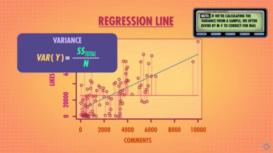
Mathematically put,

where, N is Total Number of Observations.

5. Mean Residual Deviance

Mean residual deviance (or, deviance) is a measure of goodness of fit of a model. Higher numbers always indicate bad fit. The deviance residual is the measure of deviance contributed from each observation. The deviance residuals can be used to check the model fit at each observation for generalized linear models.

If the distribution is gaussian, then mean residual deviance is equal to MSE, and when not, it usually gives a more useful estimate of error, which is why it is the default.

6. MAE – Mean Absolute Error

The Mean Absolute Error, also known as MAE, is one of the many metrics for summarizing and assessing the quality of a machine learning model. What exactly does ‘error’ in this metric mean? We do a subtraction of Predicted value from Actual Value as below:

Prediction Error → Actual Value – Predicted Value

This prediction error is taking for each record after which we convert all error to positive. This is achieved by taking Absolute value for each error as below:

Absolute Error → |Prediction Error|

Finally, we calculate the mean for all recorded absolute errors (Average sum of all absolute errors):

MAE = Average of All absolute errors

7. RMSLE – Logarithmic Error

RMSLE (Logarithmic Error) measures the ratio between actual and predicted. It can be used when you don’t want to penalize huge differences when both the values are huge numbers. Prefer this to RMSE if an under-prediction is worse than an over-prediction.

8. Residual Deviance

See #5 above (Mean Residual Deviance). Deviance is a measure of goodness of fit of a model. Higher numbers always indicates bad fit.

9. Null Deviance

The null deviance shows how well the response variable is predicted by a model that includes only the intercept (grand mean) whereas residual with inclusion of independent variables. The residual deviance is the deviance of fitted model, while the deviance for a model which includes the offset and possible an intercept term is called as null deviance.

10. AIC – Akaike Information Criterion

The Akaike information criterion is an estimator of the relative quality of statistical models for a given set of data. Given a collection of models for the data, AIC estimates the quality of each model, relative to each of the other models. Thus, AIC provides a means for model selection. AIC is founded on information theory. When a statistical model is used to represent the process that generated the data, the representation will almost never be exact; so some information will be lost by using the model to represent the process. AIC estimates the relative information lost by a given model: the less information a model loses, the higher the quality of that model.

In making an estimate of the information lost, AIC deals with the trade-off between the goodness of fit of the model and the simplicity of the model.

11. Null Degrees of Freedom

In statistics, the number of degrees of freedom is the number of values in the final calculation of a statistic that are free to vary. The number of independent ways by which a dynamic system can move, without violating any constraint imposed on it, is called number of degrees of freedom. In other words, the number of degrees of freedom can be defined as the minimum number of independent coordinates that can specify the position of the system completely.

The term is most often used in the context of linear models (linear regression, analysis of variance), where certain random vectors are constrained to lie in linear subspaces, and the number of degrees of freedom is the dimension of the subspace. The degrees of freedom are also commonly associated with the squared lengths (or “sum of squares” of the coordinates) of such vectors, and the parameters of chi-squared and other distributions that arise in associated statistical testing problems.

The null degrees of freedom is the total observations in the model minus the intercept, or n – 1.

12. Residual Degrees of Freedom

The residual degrees of freedom is n minus the number of predictors in the model, including the intercept.

Addendum: Cross-Validation

Video explanation

Just how accurate is your Einstein AI model?